For a more thorough discussion on methodology and on SPAM’s mathematical model, download a complete PDF, or browse some more documents.
Overview
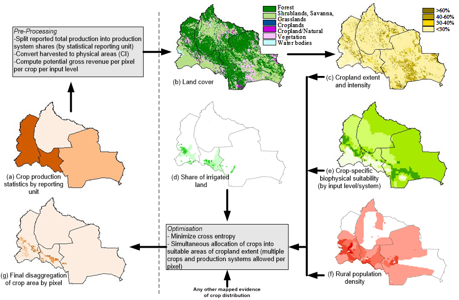
Using a variety of inputs, SPAM uses a cross-entropy approach to make plausible estimates of crop distribution within disaggregated units.
- We start with the administrative (geopolitical) units for which we have been able to obtain
 production statistics. These may typically be national or sub-national administrative regions such as countries, states, districts, or counties. The smaller the administrative units, the better the results.
 - We receive an already classified land-cover image, where cropland has been identified.
- We integrate crop-specific suitability information based on local landscape, climate and soil conditions, which provides information on how MUCH cropland exists at the pixel level.
- Combining all these input data and some more parameters the model applies a cross-entropy approach to obtain the final estimation of crop distribution.
SPAM Inputs
SPAM relies on a collection of relevant spatially explicit input data, including crop production statistics, cropland data, biophysical crop “suitability” assessments, population density, as well as any prior knowledge about the spatial distribution of specific crops or crop systems.
Some of the data is year specific, like crop statistics or population density, while other data is not really tied to a year, like suitability assessment.
Crop production statistics
While crop production data at the national level are reported by the Food and Agriculture Organization of United Nations (FAO), similar data within sub-national boundaries are rarely available on a global scale, and not from one institution. To satisfy an increasing necessity to have better crop production and land use data to support their respective programs, FAO, IFPRI (International Food Policy Research Institute) and SAGE (Center for Sustainability and the Global Environment, University of Wisconsin-Madison) started, in 2002, an informal collaborative consortium titled Agro-MAPS (Mapping of Agricultural Production Systems).
The goal of Agro-MAPS is to compile a consistent global spatial database based upon selected sub-national agricultural statistics. Agro-MAPS holds not only tabular statistical data but also links to maps of administrative districts. As input into SPAM, we started with Agro-MAPS data and made a great effort to add more sub-national data, paying particular attention to developing countries in Africa, Latin America, and Asia. We established a network of data resources from various local subnational offices in many countries throughout the world. Currently, most of the data used are from World Food Programme (WFP) crop and food supply assessment mission surveys, agricultural performance surveys, national bureaus of statistics, regional agricultural centers, ministries of agriculture, rural and extension services, regional NGOs, household services, ministries of the environment, and water resource groups.
Taking advantage of these national partners and the institutes under CGIAR (a global partnership that unites organizations engaged in research for a food secure future), we were able to compile a robust database with crop production data for more crops, and smaller administrative units than any single global collection of subnational production data currently available. These data were compiled from a variety of formats into standard spreadsheets and database files, and cover, when possible, three years around 2005.
Crops in SPAM 2005
42 crops/aggregates are included in SPAM 2005. Their definition follows FAO terminology (especially crop nes = crop not elsewhere specified). They are (with FAO code in parenthesis, except for highly aggregated crops):
Production systems
Since biophysical crop suitability or agricultural activities on any farm cannot be separated from the production system in question, we consider 4 production systems for each crop:
-
- irrigated high inputs production (I)
- rainfed high inputs production (H)
- rainfed low inputs production (L)
- rainfed subsistence production (S)
The definition of these production systems (management levels) more or less follows FAO/IIASA’s GAEZ project since we use its suitability surfaces.
Irrigated high inputs production refers to the crop area equipped with either full or partial control irrigation. Normally the crop production on the irrigated fields uses a high level of inputs such as modern varieties and fertilizer as well as advanced management such as soil/water conservation measures.
The rainfed, high input/commercial production is rainfed-based, uses high-yield varieties and some animal traction and mechanization. It at least applies some fertilizer, chemical pest, disease or weed controls and most of the product is produced for the market.
The rainfed, low-input production refers to rainfed crop production which uses traditional varieties and mainly manual labor without (or with little) application of nutrients or chemicals for pest and disease control. Production is mostly for their own consumption.
A fourth production system, rainfed, low-input/subsistence production was introduced to account for situations where cropland and suitable areas do not exist, but farmland is still present in some way.
The share of crop area and production belonging to each of these production systems when total area and production are given is often times hard to come by. In some countries there are statistics, experts may give their opinions, or assumptions are made as to how some crops are grown in a similar way as other crops.
Shares of Irrigated high input agriculture were taken directly for country statistics for China, USA, Brazil, …at sub-national administration level 1. For other countries (…) these figures were found in MIRCA and yet for the rest of the countries AQUASTAT provides information on irrigated areas per crop at the national level.
Allocation results are generated for each crop and each of the 4 production systems, however, SPAM maps and data download are only made available for irrigated and rainfed (the sum of 2, 3 and 4 above) production systems, and the sum of all, which is the total for any given crop.
Cropping intensity and multiple cropping
Estimation of crop distribution within a statistical unit is done in SPAM for the physical area. However, statistical information refers in general to harvested area, from where crops are gathered. SPAM considers 42 crops and handles each crop as if it was grown by itself on a plot, which often is not the case. In many countries, there are regions and seasons where more than one crop is grown simultaneously on one plot. Frequently there is a succession of different crops on one plot throughout the year, especially in tropical countries. All these facts are combined in a cropping intensity parameter for each crop, which is larger than 1 when there is multi-cropping, or more than one harvest per year from one plot, of different crops.
If country statistics have been prepared adequately, they will account for these conditions in the statistics and not double count areas, but this is not always the case. (Same crops on the same plot are generally reported)
Also here we rely on seldom published country statistics and lacking these expert judgments, to compile cropping intensities for each crop, which are crucial in recalculating the harvested areas to generate physical areas.
Crop suitability
Different crops have different thermal, moisture, and soil requirements, particularly under rainfed conditions. FAO, in collaboration with the International Institute for Applied Systems Analysis (IIASA), has developed the agro-ecological zones (AEZ) methodology based on an evaluation of existing land resources and biophysical limitations and potentials for specific crops (FAO/IIASA). This methodology provides maximum potential and biophysically attainable crop yields and suitable crop areas. For SPAM we utilized three production system types from the FAO/IIASA suitability datasets: Irrigated high-high input; rainfed – high input/commercial; rainfed – low input/subsistence. This latter one is also used for rainfed – subsistence farming when attainable yields are needed. For each crop and in each production systems, we define our suitable land as the sum of the four suitability classes in the AEZ model: very suitable, suitable, moderately suitable, and marginally suitable. These data were made available at a 5-minute resolution by IIASA.
For SPAM we used GAEZ’s agro-ecological productivity/total production capacity for our suitable (potential) yields for each crop and production system, and crop suitability index as a multiplier for the pixel area to receive suitable (potential) area for each crop and production system.
GAEZ only reports potential yields and suitability indices for 3 of our production systems (irrigated, rainfed high and rainfed low). For rainfed subsistence, we used the values given for rainfed low when needed.
Not all crops considered in SPAM2005 have a matching crop in the GAEZ methodology, in which case the SPAM crop ‘borrows’ from another similar GAEZ crop the attainable crop yield and suitable area.
Cropland
Satellite-based land cover datasets serve to provide detailed spatial information on cropland extent – distinguishing cropland from other forms of land cover such as forest, grassland, and water bodies and, therefore, delineating the geographical extents within which crop production must be allocated. The reliability of the land cover data in terms of measuring cropland can have significant implications for the overall reliability of the allocation.
There are several global and regional land cover datasets publicly available for various years: GlobCover 2005, MODIS v.5, AFRICOVER, GLC-2000, ISCGM, CORINE, and a number of national maps. Each dataset has its own pros and cons depending on the region of the world. Following the methodology described in Fritz et al: “Mapping Global Cropland and Field Size”, IIASA/IFPRI, 2015. all data sets were combined resulting in a global cropland map at a resolution of 30 arc seconds (approx 1x1km at the equator) and aggregated to a 5 minute (approximately 10x10km at the equator) resolution for input to the SPAM allocation.
Irrigation areas
Information on actual land use is even more difficult to find than that on cropland. One key factor to successfully allocating production statistics is to know what areas are irrigated. The Land and Water Division of FAO and the University of Frankfurt continue to work together to develop updates of the Global Map of Irrigated Areas (GMIA V5.0) which provides GIS coverage of areas equipped for irrigation at a 5-minute resolution. With this data, we were able to identify areas that were most likely irrigated and thus allocated the irrigated area and production to these locations.
Rural population density
In the absence of cropland and suitable areas, we assume that subsistence farming happens more intensively when the rural population is more abundant. For this parameter, we used rural population density as included in the GRUMPv1 data set from Columbia University and aggregated the 30 arc seconds (1x1km) to a 5 min (10x10km) grid to be used in SPAM.
Crop distribution maps
The best way to establish crop distribution in an area is not a model, like SPAM, but the actual knowledge of where crops are grown. Unfortunately, such knowledge is sparse and mostly confined to countries with highly sophisticated agriculture and monitoring systems. Expert judgment can often supplant this information, and where possible, SPAM includes such maps to force the model to allocate crop production to specific areas.
Crop distribution maps are also given at a 5 min resolution, but only available for a few crops and in some areas.
Crop prices
SPAM’s cross entropy starts with prior knowledge of where crops may be grown and to which extent. It assumes that farmers, given a choice of different crops, will grow those which generate more revenue. And this is where crop prices come in.
We use a different price for every crop, but the same price for all countries: 2004-2006 average international price, as used by FAO to compute Value of Production.
The Allocation
The allocation mechanism starts with pre-allocated areas and a number of intricate rules which are summarized below.
-
- Minimize difference between prior and allocated area share for all pixels, crops and production systems in a cross entropy equation
-
- Subject to constraints (limits) dictated by existing
- agricultural area
- irrigated area
- suitable area
- crop area statistics
- Solve in an optimization model written in GAMS
- Subject to constraints (limits) dictated by existing
All the details for this process will be found in SPAM2000 in You, L., S. Wood, U. Wood-Sichra, W. Wu. 2014. Generating global crop distribution maps: From census to grid. Agricultural Systems 127 (2014) 53–60
SPAM Outputs
After all input values have been fed into the model, SPAM returns the physical area for each crop and production system in each pixel, ie 42 x 4 values per pixel.
Using the same cropping intensity parameters as above, and further the potentially attainable yields and national/sub-national yield statistics, we further calculate area harvested, yield and production for each of the 42 crops.
Harvested area, production, and yield are modified to conform after aggregation to country level with FAO’s national values for the average 2004-2006. This adjustment is also done with the input statistics before feeding the model, the scaling of the output is repeated to level out “entropy slacks”.
Physical area (A)
Physical area is measured in a hectare and represents the actual area where a crop is grown, not counting how often production was harvested from it. Physical area is calculated for each production system and crop, and the sum of all physical areas of the four production systems constitute the total physical area for that crop. The sum of the physical areas of all crops in a pixel may not be larger than the pixel size.
Harvested area (H)
Also measured in a hectare, harvested area is at least as large as physical area, but sometimes more, since it also accounts for multiple harvests of a crop on the same plot. Like for physical area, the harvested area is calculated for each production system and the sum of all harvested areas of all production systems in a pixel amount to the total harvested area of the pixel.
The sum of all the harvested areas of the crops in a pixel can be larger than the pixel size.
Production (P)
Production, for each production system and crop, is calculated by multiplying area harvested with yield. It is measured in metric tons. The total production of a crop includes the production of all production systems of that crop.
Yield (Y)
Yield is a measure of productivity, the amount of production per harvested area, and is measured in kilogram/hectare. The total yield of a crop, when considering all production systems, is not the sum of the individual yields, but the weighted average of the 4 yields.